Your neighbors are playing Bohemian Rhapsody. Through the wall, you hear the piano, the bass and Freddie Mercury’s voice. The cymbals in the rock section lose their shimmer, because walls block high frequencies first.

Most audio-language models hear the world through a similar wall. They inherit it from Whisper, OpenAI’s speech recognition model, which deletes everything above 8 kHz before it listens. Whisper is everywhere. Hugging Face lists about 34,000 models with “whisper” in the name, and OpenAI’s two large Whisper checkpoints get about 12 million downloads a month. Audio Flamingo models have used a Whisper-based encoder since version 3.

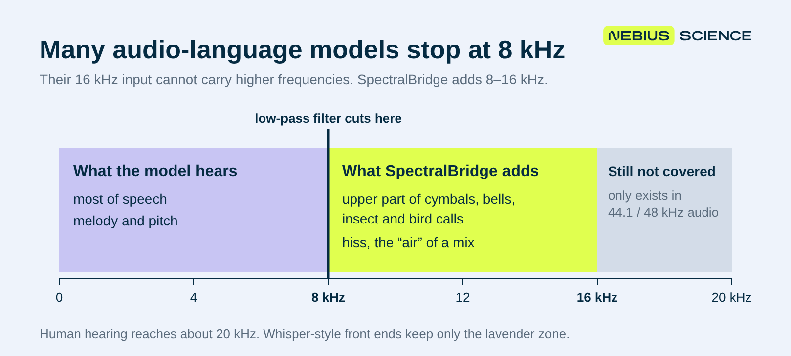
That band (8–16 kHz) carries important sound cues. Voice-cloning tools often leave errors there, and deepfake detectors look for them. Many insects call there, and ecologists track insect populations by recording their sound. A music assistant cannot judge a mix without it. Play a heavy-rain clip from a standard test set to a model that only hears up to 8 kHz, and it may answer “pouring water”. The cue that tells the two apart sits above that cutoff.

SpectralBridge, a new NeurIPS-2026 paper by Nebius researchers Sergei Polezhaev, Saba Anjum and Michael Gormish, adds that band. It trains only a small add-on and leaves the original model frozen. On an insect-species task, accuracy doubled, from 26% to 55%. The same recipe could let audio models do work they cannot do today, from bioacoustics to music production.

“It would be interesting to see the approach applied to music. Existing LLMs can’t be good music production assistants because of the 16 kHz limit, and when you create music, it is very important to hear these frequencies to analyze how a piece sounds, ” says Sergei Polezhaev, the lead author.

Why audio AI stops at 8 kHzWhy audio AI stops at 8 kHz

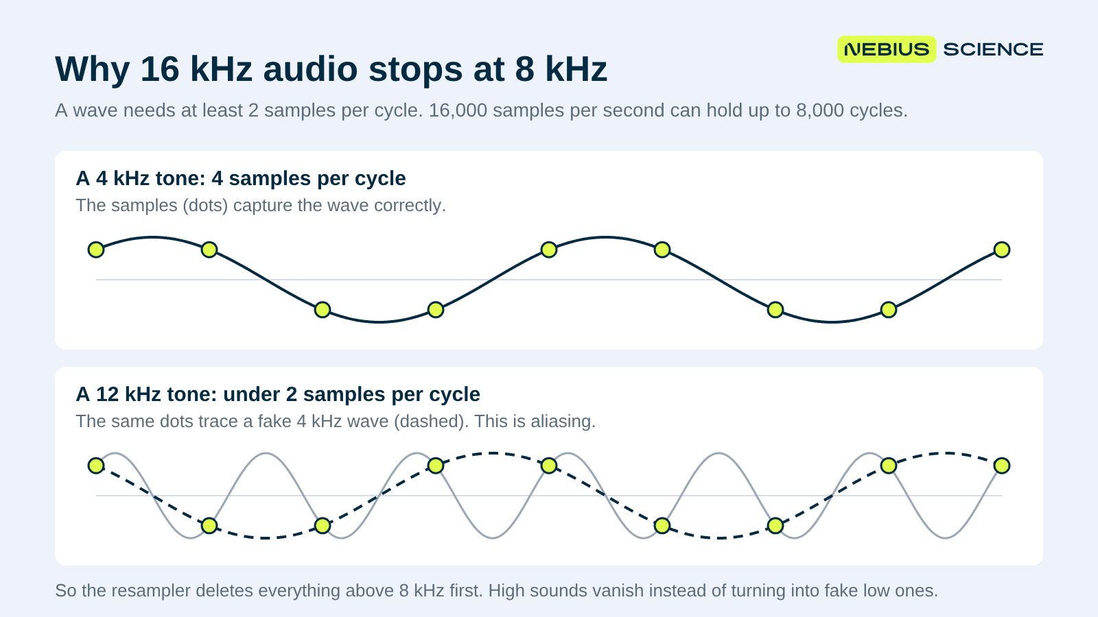
The wall comes from speech recognition. Whisper and the models built on it convert all audio to 16 kHz mono, or 16,000 samples per second.

To capture a sound wave, you need at least two samples per cycle. So 16 kHz sampling can hold sounds only up to 8 kHz. This is the Nyquist limit. Above it, the samples of a high tone trace a fake lower tone, an effect called aliasing. To prevent that, the resampler deletes everything above 8 kHz before the conversion.

Speech loses little: most of what words carry sits well below 8 kHz, and fewer samples mean less compute. Other sounds lose more. Music is recorded at 44.1 kHz or more, and human ears reach about 20 kHz. Cymbals, bells, insect calls, sibilance, hiss and the “air” of a music mix all live partly above 8 kHz.

Standard benchmarks rarely catch this. A model can often recognize a bell from its lower overtones, so a high score on a bell test says little about the upper band.

Other groups rebuild a speech model’s input layer for 16–48 kHz audio, which needs new pretraining, or add a second 48 kHz encoder next to the 16 kHz one. Audio Flamingo went the other way: starting with version 3, it replaced its higher-bandwidth encoders with a Whisper-based 16 kHz encoder, for training stability.

The open question: can a strong, frozen 16 kHz encoder still hear the octave above 8 kHz?

The trick: shift the band downThe trick: shift the band down

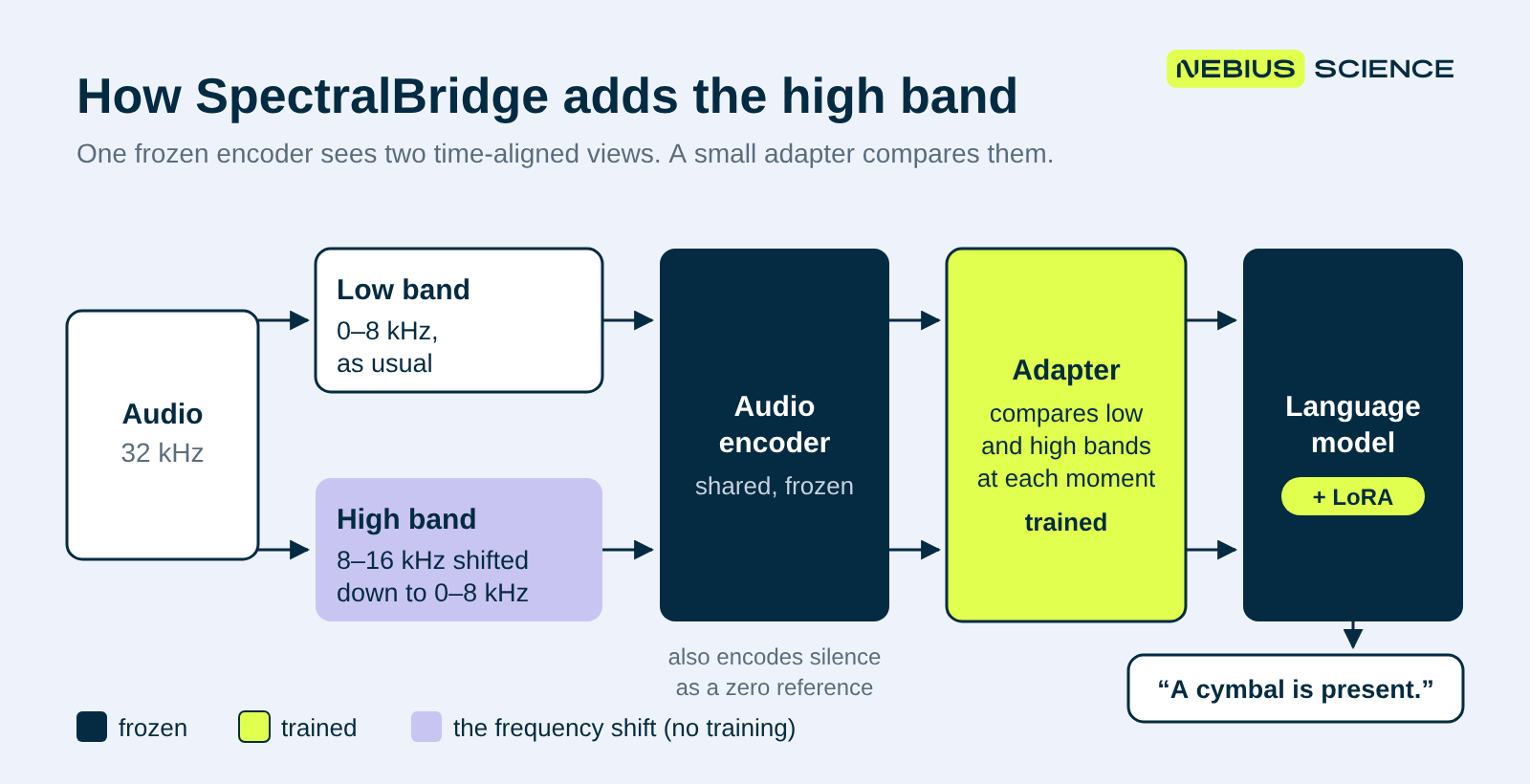
The authors start from the family’s latest model, Audio Flamingo Next, which they picked as one of the strongest open models for speech, sound and music. Its Whisper-based encoder was trained further on a large mix of speech, sound and music, so replacing it would throw that work away. Instead, they take 32 kHz audio and make two views of every clip:

• Low band, 0–8 kHz, processed as usual.
• High band, 8–16 kHz, shifted down into 0–8 kHz. The shift multiplies the signal by an 8 kHz cosine wave. This is heterodyning, and radio receivers have used it for about a century. A cricket chirp at 12 kHz reaches the encoder as 4 kHz, at the same moment in time.

Both views go through the same frozen encoder. A third pass encodes pure silence. It tells the model what the encoder outputs when the high band is empty.

A small adapter then compares the two views, one moment at a time. At each step, it sees two inputs: the low-band state, and the high-band state minus the silence reference. The more sound there is in the 8–16 kHz band at that instant, the stronger the adapter’s effect. When that band is silent, the adapter switches off completely.

Most early experiments made quality worse, and a plain LoRA baseline was hard to beat.

“At first, we wanted to modify the projector so it could handle the low and high bands without extra tokens. That gave a very small gain. Then we simply concatenated twice as many tokens and trained LoRA, and it immediately beat all our previous ideas. Processing the two bands separately helps a lot,” Polezhaev says.

Only the adapter and rank-8 LoRA modules are trained, for 600 steps on four H100 GPUs. The encoder and the 7-billion-parameter language model stay frozen. The training questions use none of the test sound classes. They cover signal physics: Was the top end of this recording cut? Which of two copies has hiss in its top octave? Which quarter of the clip has the most energy above 8 kHz? Some questions depend only on the low band, so the model does not learn that the high band always matters.

“A fully synthetic dataset worked much better than existing real sound datasets, or synthetic data made from real audio,” says Sergei.

The synthetic set was built so that only the tested property changes, for example how much energy sits above 8 kHz. Each label comes from that known change, so it is exact.

The silence testThe silence test

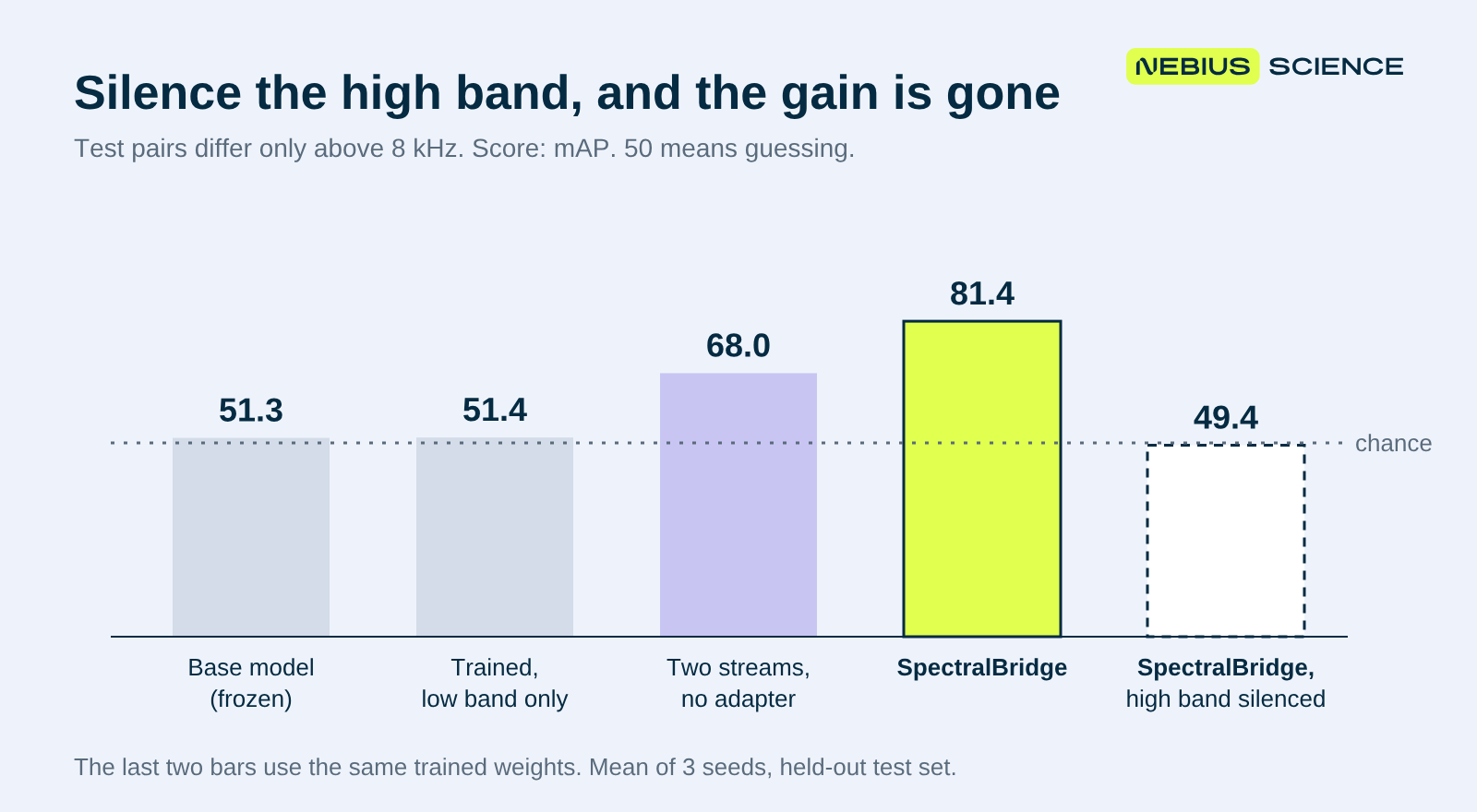
To check that the model uses the new band, the authors built test pairs from the FSD50K sound dataset. Both members of a pair are identical below 8 kHz. One has a cymbal, bell or insect added between 8 and 16 kHz. The other has a non-target sound with the same energy.

The base model scores 51.3 mAP (mean average precision, a ranking score where 50 means guessing). SpectralBridge scores 81.4. The key check: with the high band silenced, the same trained model falls to 49.4. So the gain comes from the 8–16 kHz signal, not from extra tokens or training. A simpler version gets both bands side by side, with no adapter, and reaches 68.0. So the adapter adds about 13 points.

On real recordings, the effect is smaller, because most sounds also have cues below 8 kHz. On the ESC-50 environmental sound benchmark, accuracy rises from 75.5 to 90.5. Over half of that comes from training on the answer format: a model trained on the low band only reaches 83.8.

With the high band silenced, SpectralBridge drops to 86.8, so the high band itself adds about 4 points. On one heavy-rain clip, only 6.94% of the sound’s power lies above 8 kHz. The low-band model answers “pouring water”. SpectralBridge correctly answers “rain” in all training runs, and reverts to “pouring water” when the high band is silenced.

The largest gap on real data appears after fine-tuning. On a 10-species insect task the authors built from field recordings, a low-band baseline reaches 26.2% balanced accuracy (accuracy averaged across the 10 species). SpectralBridge reaches 55.4 with the same training budget, and 22.7 with the high band silenced. On orchestral notes there is no clear gain, which fits: note identity sits mostly below 8 kHz.

Two bands mean twice the audio tokens. A compressed version pools neighboring frames back to the original count and matches the full model (83.6 vs 83.3 mAP on development data).

The fine print: the method stops at 16 kHz, so content above it, present in 44.1 and 48 kHz audio, is ignored. The method was tested on one base model only. It did not hurt the base model on two standard tests, but a wider check is still missing. Synthetic training data may invite shortcuts and limit how well the model generalizes to real recordings.

Why the high end mattersWhy the high end matters

SpectralBridge is a retrofit recipe, closer to a turbo kit than a new engine. Keep the encoder you trust, shift the missing band into its range, and train a small adapter. The test design also works for other models: pairs that differ in only one band, plus the same model with that band silenced, show whether a model uses the input you think it uses.

The applications sit where the 8–16 kHz band carries the answer. Bioacoustics needs insect and bird calls. Music tools need to judge the top end of a mix. Deepfake detection looks for traces of the vocoder, the part of a voice generator that turns its output into sound. These traces often sit in the upper band. Machine monitoring already shifts ultrasonic sensor signals into the range of pretrained audio models, as a 2026 study on hydraulic seal wear showed.

“This project is a step beyond text and opens up new research directions for Nebius,” Polezhaev says.